What is Key-Based vs Range-Based Partitioning in Databases?

Understanding Data Partitioning Strategies in Distributed Systems

Last week we covered What is Partitioning and How Indexes Work in Partitioning.

Why Partition Data?

Data is partitioned primarily for scalability. A single server has limits on CPU power, memory, disk space, and network bandwidth. As a dataset or the number of requests grows, a single server eventually becomes a bottleneck. By partitioning the data across multiple servers, the storage requirement is distributed.

Scaling Reads and Writes

The read/write query load can also be spread out. If data is partitioned effectively, a query targeting a specific piece of data must only be processed by the node(s) holding that partition rather than overwhelming a single central server. Similarly, write operations can be directed to the appropriate partition, allowing multiple writes to occur concurrently across the cluster.

Fig. Scaling Reads and Writes

Fault Tolerance

Fault tolerance is another critical benefit. If data is stored on a single machine and that machine fails, the entire dataset becomes unavailable. With partitioning, if one node fails, only the partitions it hosts become unavailable (replication strategies mitigate this). The rest of the dataset remains accessible, improving the system's overall availability and resilience.

Fig. Fault Tolerance

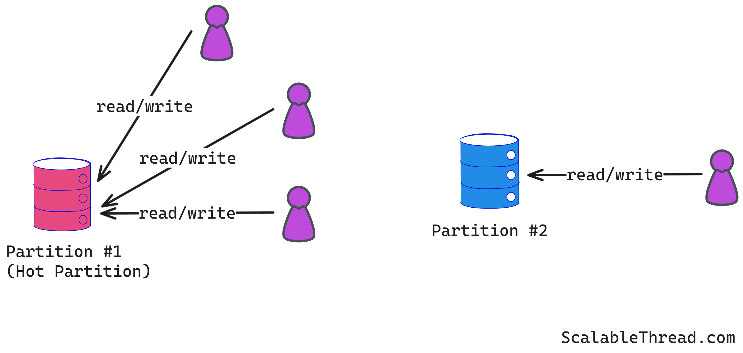
Hotspots

Achieving scalability through partitioning depends heavily on how the data is partitioned. A poorly designed partitioning strategy can lead to data skew, where some partitions store significantly more data than others. This imbalance causes hotspots.

Fig. Hot Shards

Range-Based Partitioning

Range-based partitioning involves dividing the data based on contiguous ranges of a specific attribute, known as the partition key. The system defines key ranges, each assigned to a specific partition. The partition key should be an attribute whose values have a natural order, such as timestamps, numerical IDs, or alphabetical strings.

For example, consider a database storing user information partitioned by user_id.

• Partition 1: user_id from 1 to 1,000,000

• Partition 2: user_id from 1,000,001 to 2,000,000

• Partition 3: user_id from 2,000,001 to 3,000,000

Another example could use order dates:

• Partition A: Orders placed in January 2025

• Partition B: Orders placed in February 2025

• Partition C: Orders placed in March 2025

Fig. Range-Based Partitioning

The primary advantage of range partitioning is its efficiency for range queries. Suppose an application needs to retrieve all users with IDs between 500,000 and 600,000. In that case, the system knows immediately that this data resides entirely within Partition 1. The query only needs to be routed to the node(s) holding Partition 1, significantly reducing the search scope compared to random assignment.

Susceptible to Hotspots

However, range partitioning is susceptible to creating hot spots. Specific partitions can become overloaded if access patterns are not uniformly distributed across the key ranges. In the user_id example, if newly registered users (with higher IDs) are accessed more frequently, the partitions holding the highest ID ranges will experience more load. In the order date example, if most queries target recent orders, the current month's data partition will become a hot spot for both reads and writes.

Key-Based Partitioning

Key-based partitioning aims to distribute data more evenly than range partitioning, mitigating the hot spot issues associated with predictable ranges. In this strategy, a hash function is applied to the partition key of each data record. The output of the hash function determines which partition the record belongs to. A common method is to use the modulo operator. If there are N partitions, the target partition for a record with key k might be calculated as partition = hash(k) % N.

For example, consider partitioning user data by user_id across three partitions using a hash function:

• User with user_id 123 —> hash(123) = 84362 —> 84362 % 3 = 2. The record goes to Partition 2.

• User with user_id 456 —> hash(456) = 19373 —> 19372 % 3 = 1. The record goes to Partition 1.

• User with user_id 789 —> hash(789) = 55219 —> 55221 % 3 = 0. The record goes to Partition 0.

Fig. Key-Based Patitioning

A good hash function distributes keys pseudo-randomly and uniformly across its possible output values. This ensures that each partition receives a roughly equal amount of data and request load. This approach effectively spreads write load and avoids hot spots caused by access patterns concentrating on specific key ranges.

The main disadvantage of hash partitioning is that it makes range queries inefficient. Since keys that are close together in their natural order (e.g., user_id 1000 and 1001) are likely mapped to different partitions by the hash function, retrieving a range of keys (e.g., all users with IDs between 1000 and 2000) requires querying all partitions. The relationship between adjacent keys is lost in the hashing process.

---

If you enjoyed this article, please hit the ❤️ like button.

If you think someone else will benefit from this, then please 🔁 share this post.